Decision trees and ensemble methods
This is a post I am writing to consolidate and clarify my understanding of decision trees and their ensemble methods such as bagging, boosting and forests. I used the ISLP book$^1$ (freely downloadable here) to learn this stuff so most of the content here (including much of the data and code) is a proper subset of Chapter 8 of that book.
1. What is a decision tree?
A decision tree is a supervised learning algorithm that can be used for both regression and classification. It proceeds by stratifying the dataset through a series of partitions, each of which is determined by the classification decision that needs to happen at that step. Such a partition corresponds to a node of a binary tree, where at each step a decision is being made whether to go to the left child or the right child. If this description sounds complicated, the picture below might help understand what I mean.
 Figure 1. The partitioning of the dataset corresponding to the splitting of the tree nodes
In the figure we have a simple dataset consisting of two features, a and b, and 26 samples. The samples can be classified into five different classes and the decision boundaries are what we would call piecewise constant. As you can imagine, logistic regression (i.e. linear classification) would struggle with this since the decision boundaries aren’t linear, but a decision tree is perfect. Now, obviously, “real-life” datasets are almost never this nice, so decision trees suffer from overfitting and other drawbacks, which is why we use the ensemble methods that I will come to later.
2. Building a decision tree
Let’s assume we are building a decision tree for a classification problem with $K$ classes. Decision trees, unlike many standard machine learning models, do not use a loss function to train (gradient boosted trees do; more on that later). Instead they try to optimize the “purity” of the split at each node: essentially we want the split at each node to make the starkest possible distinction between the classes we are trying to predict. A common way to measure this purity is the entropy, which should be familiar if you’ve seen Shannon entropy or Gibbs entropy before:
\[H(m) = - \sum_{k=1}^K \hat{p}_{mk} \log \hat{p}_{mk}\]where $\hat p_{mk}$ is the proportion of samples in the $m^{th}$ region that belong to the $k^{th}$ class. As the formula suggests, $H(m)$ is a nonnegative number that is minimized when all the $\hat{p}_{mk}$’s are all near 0 or near 1 i.e. the region is “pure”.
The decision tree is constructed by finding the least $H(m)$ over all possible $m$ (which means iterating over all features and trying out all possible thresholds or categories for each feature). This proceeds until a stopping criterion has reached. The stopping criterion could just be: stop when all leaves are pure. This however can lead to very complicated trees that tend to be overfitted and sensitive to variations in the input. Standard stopping criterion inlcude limiting the depth of the tree, setting lower bounds on the minimum number of samples required to split a node or to form a leaf, and requiring a minimum decrease in the impurity when splitting a node.
3. Implementing a decision tree
We are going to use the Carseats example from $\S$ 8.3.1 in [1]. First we install/import the packages we need (I’m working in Google Colab here):
!pip install ISLP
import numpy as np
import pandas as pd
from matplotlib.pyplot import subplots
from ISLP import load_data
and then load the dataset:
carseats = load_data('Carseats')
carseats.head()
which gives the output:
| Sales | CompPrice | Income | Advertising | Population | Price | ShelveLoc | Age | Education | Urban | US | |
|---|---|---|---|---|---|---|---|---|---|---|---|
| 0 | 9.50 | 138 | 73 | 11 | 276 | 120 | Bad | 42 | 17 | Yes | Yes |
| 1 | 11.22 | 111 | 48 | 16 | 260 | 83 | Good | 65 | 10 | Yes | Yes |
| 2 | 10.06 | 113 | 35 | 10 | 269 | 80 | Medium | 59 | 12 | Yes | Yes |
| 3 | 7.40 | 117 | 100 | 4 | 466 | 97 | Medium | 55 | 14 | Yes | Yes |
| 4 | 4.15 | 141 | 64 | 3 | 340 | 128 | Bad | 38 | 13 | Yes | No |
Our goal here is to predict Sales based on the other features. However since this is a continuous feature, we are going to turn this into a classification problem for classifying whether the Sales are below or above a certain threshold (i.e. a binary classification problem). Accordingly we create the output variable:
y = np.where(carseats.Sales > 8, "Yes", "No")
We make a training/validation set split:
from sklearn.model_selection import train_test_split

SEED = 20

X_train, X_test, y_train, y_test = train_test_split(
    X, y, test_size = 0.2, random_state = SEED
)
As usual, we will need to transform our features before we can train the model. In general, decision trees can work with categorical features as is, since the splits at a node can be given by whether a given categorical feature belongs to a certain category. Scikit-learn models however do not have this functionality, so we are going to need to one-hot encode our categorical features. We are going to set up a custom pipeline that we can use with multiple classifiers:
from sklearn.preprocessing import StandardScaler, OneHotEncoder
from sklearn.compose import ColumnTransformer
from sklearn.pipeline import make_pipeline
from sklearn.metrics import classification_report

numerical_features = ['CompPrice', 'Income', 'Advertising', 'Population',
    'Price', 'Age', 'Education']
categorical_features = ['ShelveLoc', 'Urban', 'US']

def custom_pipeline(classifier):
    return make_pipeline(
        ColumnTransformer([
            ('categorical', OneHotEncoder(), categorical_features),
            ('numerical', StandardScaler(), numerical_features)],
            remainder = 'passthrough',
        ),
        classifier
    )
Here’s the decision tree:
from sklearn.tree import DecisionTreeClassifier

dt = DecisionTreeClassifier(
    criterion = 'entropy',
    max_depth = 5,
    random_state = SEED
)
dt_pipe = custom_pipeline(dt)
which we train:
dt_pipe.fit(X_train, y_train)
and evaluate:
print(classification_report(y_test, dt_pipe.predict(X_test)))
to get the following results:
              precision    recall  f1-score   support

          No       0.71      0.78      0.74        46
         Yes       0.66      0.56      0.60        34

    accuracy                           0.69        80
   macro avg       0.68      0.67      0.67        80
weighted avg       0.68      0.69      0.68        80
Not exactly great. Let’s plot the learning curve to see what’s happening here.
from sklearn.model_selection import LearningCurveDisplay as LCD, ShuffleSplit

common_params = {
    "X": X,
    "y": y,
    "train_sizes": np.linspace(0.1, 1.0, 5),
    "cv": ShuffleSplit(n_splits=50, test_size=0.2, random_state=0),
    "score_type": "both",
    "line_kw": {"marker": "o"},
    "std_display_style": "fill_between",
    "score_name": "Accuracy",
}

LCD.from_estimator(
    estimator = dt_pipe,
    **common_params
)
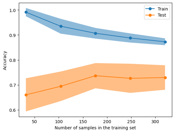 Figure 2. The learning curve display for our decision tree
The slight dip in the test score between the 150 and 200 markers could indicate overfitting. One way to deal with this problem is bagging.
4. Bagging
Bagging is the first of the ensemble methods we are going to look at. Bagging actually stands for Bootstrap AGgregation. Bootstrapping in this context refers to sampling (with replacement) subsets of the training set. The aggregation refers to the fact that we are going to aggregate the predictions of the trees (each of which has been constructed using the subsets we’ve sampled earlier). The resulting classifier can often have better properties (such as lower variance) than the original classifier. Let’s see if that is indeed the case here.
from sklearn.ensemble import BaggingClassifier

bag = BaggingClassifier(
    DecisionTreeClassifier(criterion='entropy',
        max_depth = 5,
        random_state = SEED),
    n_estimators = 10,
    max_samples = 0.5
)

bag_pipe = custom_pipeline(bag)

LCD.from_estimator(
    estimator = bag_pipe,
    **common_params
)
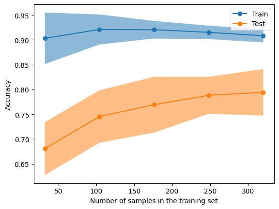 Figure 3. The learning curve for the "bagpipe"
Yes indeed! This is certainly better than the single decision tree. Note that none of this is unique to decision trees: bagging can be used with lots of other models. A natural question to ask is: if taking subsets of our samples and then aggregating learners can give better results, what about taking subsets of features instead? That’s exactly what random forests are about.
5. Random forests
Random forests overcome one of the issues with the bagging method: the one of highly correlated individual learners. This can happen when, for example, there is a feature with high importance. In such a case most of the individual trees will choose this feature for the root split and will therefore end up looking similar. Aggregating these trees then does not achieve the decrease in variance that one might have hoped for.
Random forests achieve this by selecting only a subset of the features when determining any given split. The usual size of this subset is $m = \sqrt{p}$ where $p$ is the total number of features. Of course, when $m = p$, we recover bagging. Let’s see how random forests work in our example. We shouldn’t expect much better results than previously, since we only have a handful of features to begin with, but we will see.
from sklearn.ensemble import RandomForestClassifier

rf = RandomForestClassifier(
    n_estimators = 100,
    max_depth = 5,
    criterion = 'entropy',
    max_samples = 0.5,
    random_state = SEED
)

rf_pipe = custom_pipeline(rf)
rf_pipe.fit(X_train, y_train)
print(classification_report(y_test, rf_pipe.predict(X_test)))
This gives
              precision    recall  f1-score   support

          No       0.73      0.96      0.83        46
         Yes       0.90      0.53      0.67        34

    accuracy                           0.78        80
   macro avg       0.82      0.74      0.75        80
weighted avg       0.80      0.78      0.76        80
so, yes, slightly better than bagging as we had expected, and of course quite better than the original single tree.
6. Boosting
The final ensemble method I’m going to talk about here is boosting. If one thinks of bagging or random forests as training “strong” learners in parallel, boosting can be thought of as training “weak” learners in serial. What I mean by a weak learner here is a decision tree (or some other model) that is too simple to deal with the data; it is usually underfit and misses many of the crucial relationships between the inputs and the outputs.
In a nutshell, here is how boosting works: train a weak learner on the data. Then, train the next learner on the residuals of the previous learner. We keep doing this until we reach the maximum number of weak learners, also known as estimators, or some other threshold. As can be gleaned from this informal description, boosting algorithms are sensitive to hyperparameter tuning (such as the number of estimators, the depth of each estimator, and the learning rate), and can be prone to overfitting, especially if there are stubborn samples that remain hard to infer/predict even after several iterations.
Gradient boosting and XGBoost are apparently the most widely used boosting algorithms, so I’m going to focus on those here.
6.1. Gradient boosting
Gradient boosting isn’t covered in the ISL book (as far as I can tell); I’m using the Wikipedia article and the explained.ai article$^2$ available here as references. The goal of gradient boosting is to construct a model $F_M$ where $M$ is the number of weak learners. We start off by defining $F_0$ as a very simple learner, for example $F_0$ might just predict the average output or the most common class. Assuming we’ve constructed a model $F_m$ after $m$ steps, we now train a weak learner $h_m$ on the residuals (for regression) or misclassified samples (for classification), with the goal being to minimize the loss (which can be something like mean-squared error or cross-entropy). Of course, this is the step where gradient descent comes in (hence the name). Then we set
\[F_{m+1} = F_m + \eta\, h_m\]where $\eta$ is the learning rate, one of the hyperparameters that need to be tuned. We keep doing this until we reach $m = M$. In general a higher $M$ and lower $\eta$ (i.e slow learning) yield a better model less prone to overfitting, but the cost is more training time and resources. Some variants also modify the learning rate $\eta$ after each iteration.
6.2. XGBoost
XGBoost stands for eXtreme Gradient Boosting, though the algorithm itself doesn’t use gradient descent; instead it uses Newton’s method for its optimization. The sources I’m relying on for this are mostly the Wikipedia article, the paper$^3$ XGBoost: A Scalable Tree Boosting System and the master’s thesis$^4$ Tree Boosting With XGBoost: Why Does XGBoost Win “Every” Machine Learning Competition?.
Since it uses Newton’s method, XGBoost optimizes each individual learner to fit the second-order Taylor approximation of the loss function. In particular, the loss function needs to have a second derivative (i.e. Hessian) that can be calculated and is invertible/nondegenerate. Another major way in which XGBoost differs from gradient boosting methods is in its hyperparameter $\gamma$, which determines how many leaves each tree has, as opposed to gradient boosting where each tree has the same number of nodes. This means that the individual learners are less rigid and can learn a greater range of possible relationships between the input and output variables.
XGBoost also has the hyperparameters $\alpha$ and $\lambda$ which are multiplied by the leaf weights to perform $L^1$ and $L^2$ regularization respectively. In theory these could be used for gradient boosting too, but I haven’t seen implementations doing that; it’s possible the standard XGBoost library just happens to provide robust ways of incorporating these hyperparameters that other libraries don’t.
Finally, XGBoost also implements several features that can take advantage of parallel and distributed computation, sparse data and processor caching. I am not going to go into those here, except to point out one of the core ideas of the parallelization: once we’ve split a tree node and moved to the left and right children, the subsequent splitting process at the right child can happen independently of that at the left child, and that is what the XGBoost implementation takes advantage of.
6.3. Implementing XGBoost
The XGBoost library provides interfaces/bindings for lots of different frameworks, but since we’ve been using scikit-learn so far, we’ll continue with that. We first import the necessary libraries:
from xgboost import XGBClassifier
from sklearn.preprocessing import LabelEncoder, OrdinalEncoder
and process our data:
y_processed = LabelEncoder().fit_transform(y)

X_train, X_test, y_train, y_test = train_test_split(
    X, y_processed, test_size = 0.2, random_state = SEED
)

enc = ColumnTransformer([
    ('categorical', OrdinalEncoder(), categorical_features),
    ('numerical', StandardScaler(), numerical_features)],
    remainder = 'passthrough'
)
enc.set_output(transform='pandas')
The preprocessing is different here because XGBoost actually supports categorical features, obviating the need for one-hot encoding. On the other hand, it does need the output variables to be encoded as integers, which is what the LabelEncoder is doing. We are ready to set up our model, traint it and evaluate it:
xgb = XGBClassifier(
    n_estimators = 100,
    learning_rate = 1,
    reg_alpha = 0.5,
    reg_lambda = 0.9,
    max_depth = 1,
    objective = 'binary:logistic',
    random_state = SEED,
    enable_categorical = True
)

xgb_pipe = make_pipeline(enc, xgb)

xgb_pipe.fit(X_train, y_train)

print(classification_report(y_test, xgb_pipe.predict(X_test)))
As you can see, there a lot of hyperparameters here. I’ve selected the ones that work best for this problem (after some trial-and-error). Here are the results:
              precision    recall  f1-score   support

           0       0.87      0.98      0.92        46
           1       0.96      0.79      0.87        34

    accuracy                           0.90        80
   macro avg       0.91      0.89      0.89        80
weighted avg       0.91      0.90      0.90        80
A great improvement! Observe that the max_depth of each individual learner is just 1 here, which means these are really weak learners. The resulting model still outperforms everything we’ve seen so far by a signficant margin. I highly recommend XGBoosting for more examples and how-tos on XGBoost.
7. Conclusion
Let’s summarize what we’ve learned here. Decision trees are supervised learning models that can be used for both regression and classification. They work well when the decision boundaries are piecewise linear. One of their main hyperparameters is the maximum tree depth. The larger this is, the more flexible the tree is, but also the more likely to be overfit (as with most situations involving the bias-variance tradeoff). One of the main advantages of decision trees is their interpretability. Unlike other models such as neural networks which have “hidden layers” and often operate as blackboxes, decision trees can be inspected to gauge their decision-making processes, which makes them an important option to consider when looking for an “explainable AI”. For example, here is the entire decision tree as a diagram from our first model:
from sklearn.tree import plot_tree, export_text

fig, ax = subplots(
    figsize = (60, 30)
)

plot_tree(
    dt_pipe.named_steps['decisiontreeclassifier'],
    ax = ax,
    class_names = ['No', 'Yes'],
    feature_names = [x.split('__')[-1] for x in dt_pipe[:-1].get_feature_names_out()],
    filled = True
)
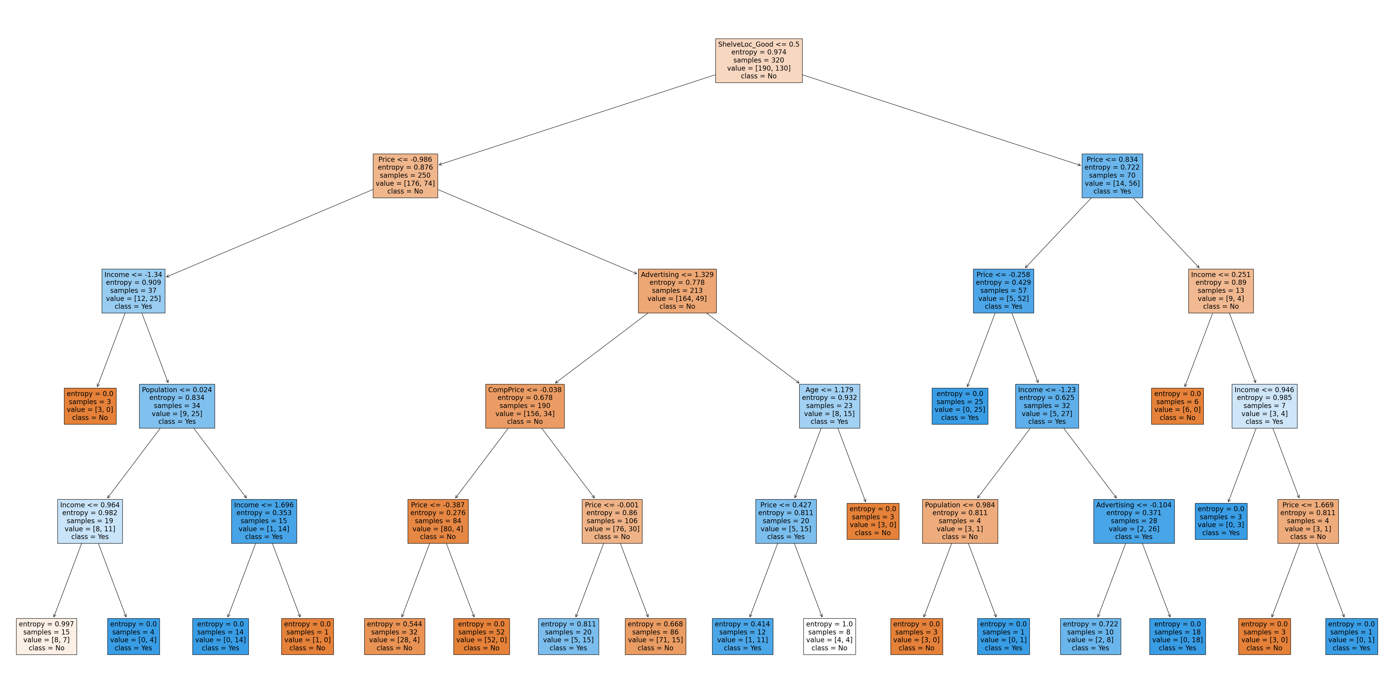 Figure 4. The entire decision tree which demonstrates how the model makes its predictions (click to zoom)
Depending on where you are viewing this, the entire picture might not be displayed. You can click on it to zoom in.
Decision trees can suffer from high variance, a drawback which can be handled using ensemble methods. The downside of these is the lack of explainability. The ones we discussed fit into two broad categories: random forests and boosting.
Random forests involve building several strong learners (i.e. complicated trees) independently on subsets of the data (drawn with replacement), with each split being decided with only a subset of the features. These sampling methods serve to decorrelate the trees and make the aggregate model more robust. As a result, random forests are less prone to overfitting. They also retain some of the interpretability of decision trees, since the final prediction is just a vote/aggregation of the individual predictions.
Boosting models, on the other hand, build several weak learners in serial, with each subsequent learner being trained on the residuals of the previous one. Several hyperparameters, such as regularization of the leaf weights, depths of individual trees, and total number of trees, can be fine-tuned to achieve a balance of the bias-variance tradeoff. Gradient boosting uses gradient descent, while XGBoost uses Newton’s method. As a consequence, XGBoost can be limited in the loss functions it can use, but can achieve better accuracy since it is a second-order approximation.
XGBoost also has a lot of built-in features that make it extremely fast and efficient, as well as adept at dealing with sparse/missing data. It is also capable of dealing with class imbalances, since subsequent learners will try to make up for the failure of a given learner to predict a rare class. On the other hand, XGBoost sacrifices explainability and the ability to figure out feature importance. It can also be overfit if the hyperparameters are not tuned properly (and tuning hyperparameters can sometimes be more of an art than a science)
References
-
James, Gareth, Daniela Witten, Trevor Hastie, Robert Tibshirani, and Jonathan Taylor. An Introduction to Statistical Learning: with Applications in Python. Springer Nature, 2023.
-
Terence Parr and Jeremy Howard. How to explain gradient boosting.
-
Tianqi Chen and Carlos Guestrin. XGBoost: A Scalable Tree Boosting System. Proceedings of the 22nd ACM SIGKDD International Conference on Knowledge Discovery and Data Mining (KDD ‘16). 2016.
-
Didrik Nielsen. Tree Boosting With XGBoost: Why Does XGBoost Win “Every” Machine Learning Competition?. MS thesis. NTNU. 2016.